Tracking the ZAR BTC USD arbitrage rate
Back in 2020 a friend told me about the USD - ZAR - BTC arbitrage. The basic idea is that the ZARBTC price is usually a little but higher than the USDZAR + USDBTC price. The reason for this is that South African Reserve Bank imposes a R10m cap on capital withdrawals from the country.
What this means is that the USDZAR leg of the trip is supply constrained, resulting in a shortage of USDZAR + USDBTC trades, which keeps the ZARBTC premium more or less permanent.
In 2021 I thought I’d investigate this claim and spent a few weekends trying to calculate the actual premium to see if I could make a bit of money on the side.
There are a few companies out there that exploit this abitrage as a service for clients, but they generally take a large cut of the profits and it seemed silly to hand over good money for something that can probably be automated over a couple of weekends.
It turns out that the devil is in the details when computing the premium in a realistic manner, so I thought I’d make a short blog post on the subject.
Obtaining Data
In order to compute the premium, you need the USDZAR, USDBTC and ZARBTC rates. Not just any rates, mind you, but the rates quoted by the actual exchanges you might trade on.
For the crypto rates, I poll Luno, and Kraken, because they are the exchanges I trade on. You can use whichever exchanges you choose, but after several weeks of research I found these two exchanges to be the best options.
The currency quotes are harder; in the end I just stick with yahoo finance because they at least provide a spread rather than a point estimate.
I generally poll these data sources every 15 minutes or so and cache the results to disk.
A note on spreads and fees
A naive calculation would just get the last traded price on each pair and then chain them together to get the implied rate. This is probably what the abovementioned arbitrage services do when they give you a ‘live potential return’ computation.
But that’s not how trades work. All exchanges provide a bid and an offer price for a particular asset. The actual trade price will be some random number between the bid and offer, and you can’t assume it will be the midpoint. If you want to be really conservative, you should model the worst outcome in your computation. If you want to be a bit more realistic, you could take a random value between the bid and offer.
Then there are fees. Broker fees. SWIFT fees. Exchange fees. Withdrawal fees. You need to incorporate these into your computation otherwise your estimates will be off. And when we are talking sub-percentage point returns these fees mean the diffeence between profit and loss.
Some Scraper Code
Ok, let’s look at some code. Here’s my yahoo-usdzar.R scraper script.
What is does is it hits the yahoo finance web page, parses the HTML, and
saves the relevant details to a csv file.
suppressMessages({options(scipen = 999)
library(rvest)
library(dplyr)
library(magrittr)
library(tidyr)
library(readr)})

# USDZAR
html <- read_html("https://finance.yahoo.com/quote/USDZAR=X")
dirname <-  "data/yahoo/USDZAR"
timestamp <- round(as.numeric(as.POSIXct( Sys.time() ))*1000,0)
dir.create(dirname, recursive = TRUE, showWarnings = F)

html %>%
  html_element("#quote-summary") %>%
  html_table() %>%
  as_tibble() %>%
  mutate(X2 = as.numeric(X2)) %>%
  select(X2) %>%
  t() %>% as_tibble(.name_repair = "minimal") %>%
  set_colnames(c("prev_close", "open", "bid", "day_range", "52wk_range", "ask")) %>%
  select(-day_range, -`52wk_range`) %>%
  mutate(client_timestamp = timestamp) %>%
  write.table("data/yahoo/USDZAR/data.csv",
              append = TRUE,
              sep = ",",
              dec = ".",
              row.names = FALSE,
              col.names = FALSE)
## Warning in mask$eval_all_mutate(quo): NAs introduced by coercion
Here’s what that csv file looks like.
glimpse(read.csv("data/yahoo/USDZAR/data.csv"))
## Rows: 15,546
## Columns: 5
## $ prev_close       <dbl> 15.8713, 15.8713, 15.8713, 15.8713, 15.8713, 15.8713,…
## $ open             <dbl> 15.8760, 15.8760, 15.8760, 15.8760, 15.8760, 15.8760,…
## $ bid              <dbl> 15.6995, 15.7034, 15.7748, 15.7508, 15.7550, 15.7550,…
## $ ask              <dbl> 15.7095, 15.7063, 15.7787, 15.7556, 15.7650, 15.7650,…
## $ client_timestamp <dbl> 1641480848064, 1641480858387, 1641501776072, 16415029…
Next we hit the Luno API for the ZARBTC rate. Here’s what my
luno-xbtzar.R script looks like.
suppressMessages({library(httr)
library(tibble)})

file <- "data/luno/XBTZAR/data.csv"

dir.create(dirname(file), recursive = T, showWarnings = F)

timestamp <- round(as.numeric(as.POSIXct( Sys.time() ))*1000,0)

response <- GET('https://api.mybitx.com/api/1/ticker?pair=XBTZAR')
response_content <- content(response)
as_tibble(response_content) %>%
mutate(client_timestamp = timestamp) %>%
  write.table(file,
              append = TRUE,
              sep = ",",
              dec = ".",
              row.names = FALSE,
              col.names = FALSE)
And this is what that dataset looks like.
glimpse(read.csv("data/luno/XBTZAR/data.csv"))
## Rows: 15,519
## Columns: 8
## $ pair                   <chr> "XBTZAR", "XBTZAR", "XBTZAR", "XBTZAR", "XBTZAR…
## $ timestamp              <dbl> 1641502773557, 1641502933453, 1641503792792, 16…
## $ bid                    <dbl> 697516, 697264, 695795, 695829, 696461, 695522,…
## $ ask                    <dbl> 697517, 698378, 696973, 696948, 696999, 696569,…
## $ last_trade             <dbl> 697710, 697436, 696977, 696951, 696500, 695517,…
## $ rolling_24_hour_volume <dbl> 313.0051, 310.5169, 307.1836, 307.1836, 307.183…
## $ status                 <chr> "ACTIVE", "ACTIVE", "ACTIVE", "ACTIVE", "ACTIVE…
## $ client_timestamp       <dbl> 1641502773557, 1641502933453, 1641503792792, 16…
Finally we hit Kraken for the USDZAR leg.
suppressMessages({library(httr)})

file <- "data/kraken/XXBTZUSD/data.csv"

dir.create(dirname(file), recursive = T, showWarnings = F)

timestamp <- round(as.numeric(as.POSIXct( Sys.time() ))*1000,0)

response <- GET('https://api.kraken.com/0/public/Ticker?pair=XXBTZUSD')
response_content <- content(response)
result <- response_content$result
if (length(result) != 0) {
  # do some processing
  XXBTZUSD <- result$XXBTZUSD
  ask <- as.numeric(XXBTZUSD$a[[1]])
  bid <- as.numeric(XXBTZUSD$b[[1]])
  last <- as.numeric(XXBTZUSD$c[[1]])
  volume <- as.numeric(XXBTZUSD$v[[1]])
  vwap_today <- as.numeric(XXBTZUSD$p[[1]])
  num_trades_today <- as.numeric(XXBTZUSD$t[[1]])
  low_today <- as.numeric(XXBTZUSD$l[[1]])
  high_today <- as.numeric(XXBTZUSD$h[[1]])
  paste(timestamp,ask,bid,last,volume,vwap_today,num_trades_today,low_today,high_today,sep=",") %>%
  write(file,
        append = T)

}
Here’s what that data looks like.
glimpse(read.csv("data/kraken/XXBTZUSD/data.csv"))
## Rows: 15,500
## Columns: 9
## $ client_timestamp <dbl> 1641501618894, 1641501671177, 1641502930523, 16415037…
## $ ask              <dbl> 43183.6, 43159.5, 43215.1, 43159.4, 43159.4, 43182.5,…
## $ bid              <dbl> 43183.5, 43151.2, 43215.0, 43159.3, 43159.3, 43182.4,…
## $ last             <dbl> 43183.6, 43151.1, 43215.0, 43159.4, 43159.4, 43182.5,…
## $ volume           <dbl> 4354.01342530, 4358.90452901, 4399.02987492, 4418.292…
## $ vwap_today       <dbl> 43107.72, 43107.77, 43108.50, 43108.88, 43108.88, 431…
## $ num_trades_today <int> 34448, 34485, 34851, 35054, 35059, 35073, 35168, 3517…
## $ low_today        <dbl> 42424.0, 42424.0, 42424.0, 42424.0, 42424.0, 42424.0,…
## $ high_today       <dbl> 43748.0, 43748.0, 43748.0, 43748.0, 43748.0, 43748.0,…
Plotting the Raw Data
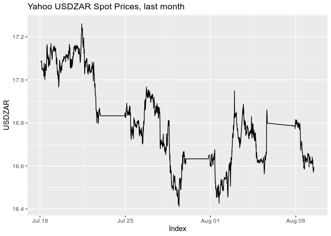
Ok, so we can log the relevant rates. Now we need to compute the estimated round trip return. Let’s read in the USDZAR data and plot it on a timeseries chart.
You’ll notice that there are some gaps in the data. These are the periods when my server was off due to load shedding rotations in my suburb.
# yahoo USDZAR
file_path <- "data/yahoo/USDZAR/data.csv"
yahoo_usdzar <- fread(file_path)

time_component <- as.POSIXct(as.numeric(yahoo_usdzar$client_timestamp)/1000, origin="1970-01-01")

data_component <- yahoo_usdzar %>%
  select(bid, ask) %>%
  rename(yahoo_bid = bid,
         yahoo_ask = ask) %>%
  mutate(across(everything(), as.numeric))

yahoo_usdzar <- xts(data_component, order.by=time_component)

yahoo_plot <- yahoo_usdzar %>% last("4 weeks") %>%
  ggplot(aes(x = Index, y = yahoo_ask)) +
  geom_line()  +
  scale_y_continuous(name = "USDZAR") +
  ggtitle('Yahoo USDZAR Spot Prices, last month')

yahoo_plot
# kraken XXBTZUSD
kraken_xbtusd <- fread("data/kraken/XXBTZUSD/data.csv")
time_component <- as.POSIXct(as.numeric(kraken_xbtusd$client_timestamp)/1000, origin="1970-01-01")
data_component <- kraken_xbtusd %>%
select(bid, ask, last) %>%
rename(kraken_bid = bid,
kraken_ask = ask,
kraken_spot = last) %>%
mutate(across(everything(), as.numeric))
kraken_xbtusd <- xts(data_component, order.by=time_component)
kraken_plot <- kraken_xbtusd %>% last("4 weeks") %>%
ggplot(aes(x = Index, y = kraken_spot)) +
geom_line() +
scale_y_continuous(name = "Kraken Spot") +
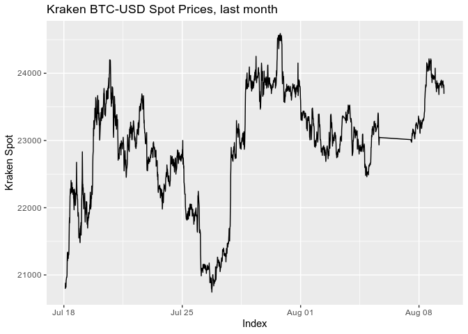
ggtitle('Kraken BTC-USD Spot Prices, last month')
kraken_xbtusd <- transform(kraken_xbtusd, kraken_spread = (kraken_ask/ kraken_bid - 1)*10000) %>% as.xts
kraken_plot
# luno XBTZAR
dir_path <- "data/luno/XBTZAR"
luno_xbtzar <- do.call(rbind,lapply(list.files(dir_path, full.names = T),fread))

time_component <- as.POSIXct(as.numeric(luno_xbtzar$client_timestamp)/1000, origin="1970-01-01")
data_component <- luno_xbtzar %>% select(bid, ask, last_trade) %>%
  rename(luno_bid = bid,
         luno_ask = ask,
         luno_last = last_trade) %>%
  mutate(across(everything(), as.numeric))
luno_xbtzar <- xts(data_component, order.by=time_component)

luno_plot <- luno_xbtzar %>% last("4 weeks") %>%
  ggplot(aes(x = Index, y = luno_last)) +
  geom_line()  +
  scale_y_continuous(name = "Luno Last") +
  ggtitle('Luno BTC-ZAR Last Trade Price, last month')

luno_xbtzar <- transform(luno_xbtzar, luno_spread = (luno_ask/ luno_bid - 1)*10000) %>% as.xts

luno_plot
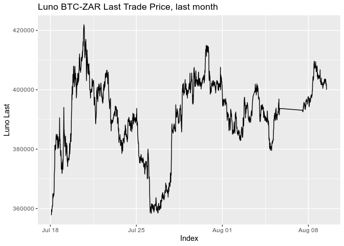
So far so good.
Computing the Premium
Let’s chain these together to compute the arbitrage premium. There are a few hard coded parameters here that are the result of good old fashioned manning-the-phones research. I’ll explain those in comments in the code as we proceed.
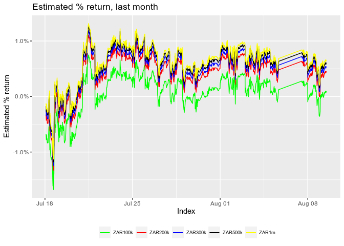
You’ll notice that I model the return for a range of invested amounts. This is because some of the costs associated with a real-world trade are fixed, and so the return will increase as you increase the invested amount.
# Potential profit ----
timestamp <- round(as.numeric(as.POSIXct( Sys.time() ))*1000,0)
# principal invested in ZAR
principals <- c(100000, 200000, 300000, 500000, 1000000)
Here we model the potential return from a round trip. I model the return conservatively by assuming I act as a price taker in the market, always just taking the offered or bid value of the asset (whichever is appropriate). Because of this, you can consider this a conservative estimate.
result <- timestamp
for (principal in principals) {
  # if you invest more than R100k, SWIFT fee is R550, if more than R100k, it's R450.
  fee <- ifelse(principal > 100000, 450, 550)
  # broker spread is .5%. Check that with your broker.
  broker_spread <- 0.005

  interbank_usdzar_rate <- median(last(yahoo_usdzar$yahoo_ask, '1 day'), na.rm = T)
  broker_usdzar_rate <- interbank_usdzar_rate * (1+broker_spread)
  principal_usd <- (principal - fee) / broker_usdzar_rate

  # from kraken fees website
  kraken_usd_deposit_fee <- 0
  kraken_usd_net <- principal_usd - kraken_usd_deposit_fee

  # from kraken fees website
  kraken_commission <- 0.0026
  kraken_usdbtc_rate <- median(last(kraken_xbtusd$kraken_ask, "1 day"), na.rm = T)
  kraken_btc <- principal_usd / kraken_usdbtc_rate / (1+kraken_commission)

  # from kraken fees website
  kraken_btc_withdrawal_fee <-  0.00015
  luno_btc <- kraken_btc - kraken_btc_withdrawal_fee

  # from luno websitre
  luno_commission <- 0.001
  luno_btczar_rate <- median(last(luno_xbtzar$luno_bid, "1 day"), na.rm = T)
  luno_zar_net <- luno_btc * luno_btczar_rate /(1+luno_commission)
  luno_withdrawal_fee <- 0
  bank_zar_net <- luno_zar_net - luno_withdrawal_fee
  bank_zar_net

  overall_return <- bank_zar_net / principal - 1
  overall_return
  result <- c(result, overall_return)
}

# Write out to file
write(paste(result, collapse = ","), "data/arbitrage/zarbtc_estimated_return.csv", append = T)
Here’s what the estimated return dataset looks like.
glimpse(read.csv("data/arbitrage/zarbtc_estimated_return.csv"))
## Rows: 14,784
## Columns: 6
## $ timestamp <dbl> 1642946176287, 1642946286511, 1642946411033, 1642946958904, …
## $ ZAR100k   <dbl> 0.01325689, 0.01300720, 0.01415953, 0.01403507, 0.01391006, …
## $ ZAR200k   <dbl> 0.01698851, 0.01673804, 0.01789604, 0.01777021, 0.01764385, …
## $ ZAR300k   <dbl> 0.01789248, 0.01764184, 0.01880134, 0.01867510, 0.01854833, …
## $ ZAR500k   <dbl> 0.01861566, 0.01836487, 0.01952557, 0.01939901, 0.01927191, …
## $ ZAR1m     <dbl> 0.01915804, 0.01890715, 0.02006875, 0.01994194, 0.01981459, …
We can plot this dataset as well.
# Plot potential profit
file_path <- "data/arbitrage/zarbtc_estimated_return.csv"
zarbtc_estimated_return <- fread(file_path)

time_component <- as.POSIXct(as.numeric(zarbtc_estimated_return$timestamp)/1000, origin="1970-01-01")
data_component <- zarbtc_estimated_return %>% select(starts_with("ZAR"))
zarbtc_estimated_return <- xts(data_component, order.by=time_component)

estimated_return_plot <- zarbtc_estimated_return %>%
  last("4 weeks") %>%
    ggplot(aes(x = Index)) +
   geom_line(aes(y = ZAR100k, color = "ZAR100k")) +
  geom_line(aes(y = ZAR200k, color = "ZAR200k")) +
  geom_line(aes(y = ZAR300k, color = "ZAR300k")) +
  geom_line(aes(y = ZAR500k, color = "ZAR500k")) +
  geom_line(aes(y = ZAR1m, color = "ZAR1m")) +
  scale_colour_manual("",
                      values = c("ZAR100k"="green", "ZAR200k"="red",
                                 "ZAR300k"="blue", "ZAR500k"="black", "ZAR1m"="yellow")) +
    scale_y_continuous(name = "Estimated % return",labels = scales::percent) +
    ggtitle('Estimated % return, last month')  +
theme(legend.position = "bottom",
      legend.title = element_text( size=7),
      legend.text=element_text(size=7))

estimated_return_plot
Evaluating the results
You can see (as of now, mid 2022) that the return for R100k is pretty low - the small traders are really not doing great. You need to get above R300k to make anywhere near 0.5%. Back in 2021 the R300k return was more like 1.5%, and back in 2019 my impression was that it was around 3%.
In 2021 I actually opened the relevant accounts and did a few test runs of this arbitrage. I’ve build a set of trading scripts that automate the BTC legs of the trade, but the actual forex purchase has to be done by emailing a trader.
My experience was that the above estimated return code was generally accurate, but conservative. So pretty good all round.
Making 1% on a R300k round trip equates to about R3k per round, and the round trip takes about 7 hours. 6.5 hours for the USD to land in Kraken, and 30 minutes for the trades to cascade down to ZAR sitting in Luno ready for withdrawal.
This feels like easy money (once you’ve automated it all) for the first 3 trades, because the South Africas Revenue Service lets you send up to R1m out of the country without and administrative overhead.
However, for the next R10m (i.e 33 trades, potentially ), you have to obtain specific permission from the South African Revenue Service, and they only give you permission for whatever you have in your account (i/e R300k at a time), and they need you to supply 3 years of income and asset declarations to apply.
This is too much admin for me, personally, and at any rate I don’t like making such comprehensive declarations to SARS. So, ofr now, my trader sits idle.
I have wrapped the above premium estimation code into an emailer which sends me a summary each morning. Maybe one day the spreads will widen again, and it’ll become worth it.