Computing adjusted prices for equity backtesting
I must confess. Even though my masters thesis was to build an equity strategy backtester, I sort of glossed over how to compute adjusted prices. I figured that I should focus on the mechanics of building a working trading engine, and that I could feed it well-vetted pricing data at some future point in time.
Well, folks, that time has come.
Why would you want to adjust prices?
Take a look at this plot of the AAPL share price from June 2014 to Oct 2022. Looks pretty dire, right? What the heck happened in mid 2020?
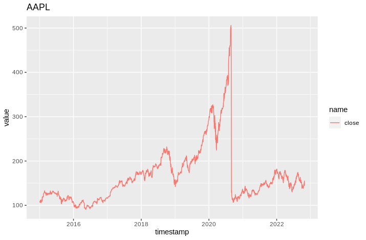
It turns out that AAPL made a 4:1 stock split in 2020. So, if you had 1000 AAPL shares the one day, you had 4000 the next. But the value of the company as a whole didn’t change, so the share price trading on the market halved.
If you were to backtest against these unadusted prices you’d end up with spurious results.
Here is the adjusted share price plot for AAPL:
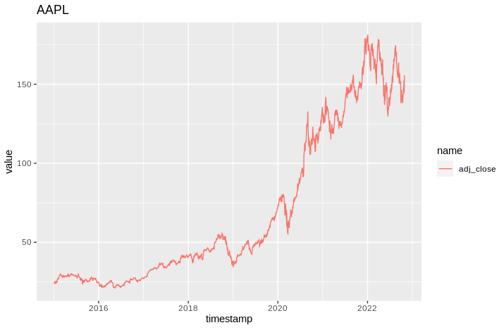
That accords more closely with reality.
How to interpret adjusted prices
The ratio between the raw, unadjusted price and the adustment price is aclled the adjustment factor. The most recent adjusted price should be the same as the raw price, i.e the adjustment factor is 1.
As you go back in time, the adjustment factor will change to incorporate changes to shares in issue, and dividend distributions. So, if a stock splits 4 for 1, your adjustment factor will go from 1 to 0.25. That means the raw prices before that date will be multiplied by 0.25 to make them comparable to your current prices. The adjusted price time series represents the total return of a stock up until the most recent observation. The raw price time series represents the price for which a stock was traded on a particular day.
Usually, when backtesting or assessing performance you care about the adjusted price, not the raw price history.
How to compute adjusted prices
Well, you could get your adusted prices from a vendor, like Bloomberg or Polygon or Alphavantage or whatever. But, even if you do that, you probably want to double check the values.
In order to compute the adjusted close, you need
- Close price each day
- Any dividends distributed each day
- Any share splits each day
You can usually get these from a data vendor. Here’s what a selection of AAPL’s TIME_SERIES_DAILY_ADJUSTED data looks like from Alphavantage:
    timestamp  close    volume adjusted_close dividend_amount split_coefficient
1  2022-10-28 155.74 164762371       155.4816               0                 1
2  2022-10-27 144.80 109180150       144.5597               0                 1
3  2022-10-26 149.35  88436172       149.1022               0                 1
4  2022-10-25 152.34  74732290       152.0872               0                 1
5  2022-10-24 149.45  75981918       149.2020               0                 1
6  2022-10-21 147.27  86548609       147.0256               0                 1
7  2022-10-20 143.39  64521989       143.1521               0                 1
8  2022-10-19 143.86  61758340       143.6213               0                 1
9  2022-10-18 143.75  99136610       143.5115               0                 1
10 2022-10-17 142.41  85250939       142.1737               0                 1
The split coefficient is the ratio of issued stock on a day relative to the day before. The dividend amount is the amount of dividends received that day.
What you want to do is ‘deflate’ each close price by the split coefficient and dividend amount of the next day. Why?
Well, the split coefficient is easy. It ’normalises’ the price so that it’s comparable to the price after the split. The dividend amount is for a different reason. Basically, what we care about is the total return from a stock. When a stock distributes a dividend, we receive that money. In a really efficient market, the price should adust to reflect that the dividend was distributed, i.e, a $10 stock that gives me $1 in dividends is not worth $9. So we want to ‘add back’ that $1 to the price to make the adjusted price more accurately reflect the total return.
Ok, how do we do that in code? I’m just going to give it to you straight up, because I took ages to wrangle it and I want to present it in a single beautiful code chunk.
library(alphavantager)
library(dplyr)
library(purrr)
# Pull adjusted data from Alphavantage
av_get(symbol = "AAPL",
                 av_fun = "TIME_SERIES_DAILY_ADJUSTED",
                 outputsize = "full") |>
# Filter to my backtest period
filter(timestamp > as_date("20150101")) |>
# Arrange from most recent to least recent
arrange(desc(timestamp))|>
# Compute split factor. This is the cumulative deflator attributable
# to splits
mutate(split_factor = accumulate(lag(split_coefficient, default  = 1), `/`)) |>
# Compute the dividend factor. This is the cumulative factor attributable
# to dividend distributions
mutate(dividend_deflator = (close - lag(dividend_amount, default = 0)) / close) |>
mutate(dividend_factor = accumulate(dividend_deflator, `*`)) |>
# Use the factors to adjust the close
mutate(my_adjusted_close = close * split_factor * dividend_factor) |>
# neaten up for display purposes
select(timestamp, close, adjusted_close, my_adjusted_close)
Which gives (the red line is covered by the blue line):
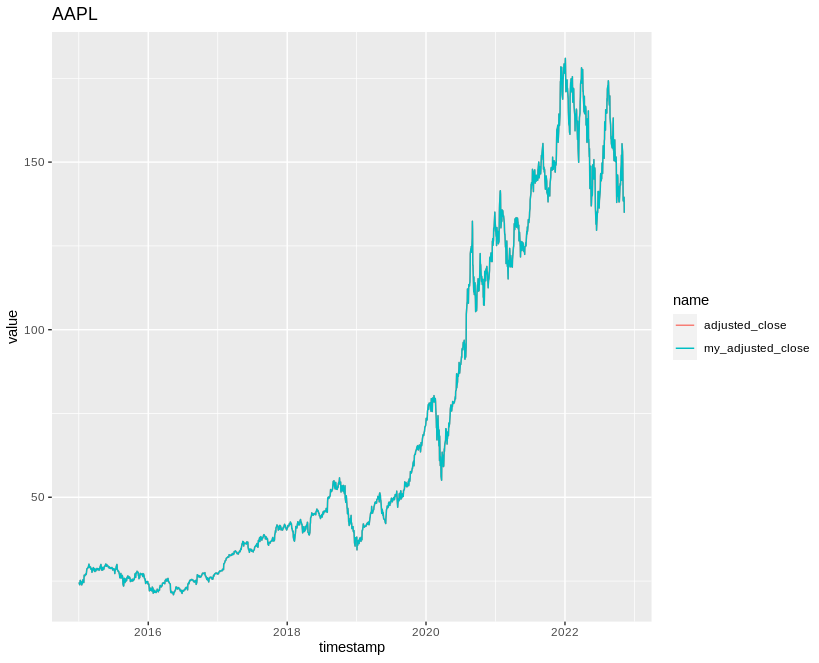
Viola! Exactly the same data we got from Alphavantage.