Checking AB test session data for interaction effects
I have been working on an AB testing platform for a client. They have quite a large site, and are running anywhere from 50-75 experiments simultaneously at any one time. Naturally, they were concerned that experiments might affect each other, so we put together a pipeline to automatically check for interaction effects.
I’ve put this blog post together because the internet resources I used to build the pipeline (deadlink: vista.io) have become deadlinks and I want to preserve the reasoning somewhere.
So, buckle up, in 10 minutes or so you’ll go from knowing nothing about AB testing to knowing more than most.
What is an experiment?
For the purposes of this post you can consider an ’experiment’ to be roughly analogous to a medical double blind study. Every time someone visits the site, they start a session, which will end when they close the tab. All their behaviour is logged to the session ID. As soon as their behaviour triggers the conditions specified in a particular experiment, they are enrolled in that experiment and are randomly assigned to either the test group or the control group.
The sessions in the test group will be shown the ’new’ version of some element of the site, and the sessions in the control group will be shown the ‘old’ (unchanged) element of the site. This element can be as simple or as complex as the experimenter likes.
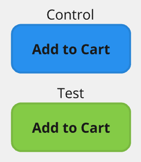
Consider an e-commerce ‘Add to Cart’ button. Let’s say that it is blue, and the font is black. An experimenter could decide to show the ’test’ group a green button instead, and then observe whether the test or control groups outperform on a chosen metric, such as the probability of adding an item to the cart.
If the test group has a statistically significant uplift for the ‘add to basket’ metric over the control baseline, we can roll the green button out to everyone and enjoy a free uplift in cart additions.
What is a metric interaction?
If you are running multiple experiments on a site concurrently, you have the risk of collision. That is to say, some experiments might interfere with other experiments in such a way that the results are skewed.
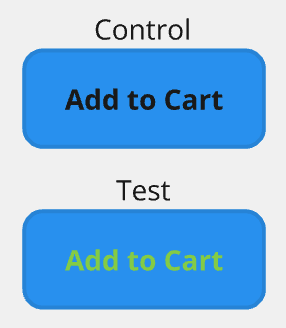
Consider our Blue/Green button experiment above. Let’s say that, unbeknownst to our experimenters (let’s call them the Button Team), the Font Team has decided that perhaps a green font will increase the probability of an Add To Cart event.
It should be obvious to you that weirdness will result if a session is enrolled in both of these experiments. Depending on the particular test/control groups it gets assigned to, here is what the Add To Cart button will look like:
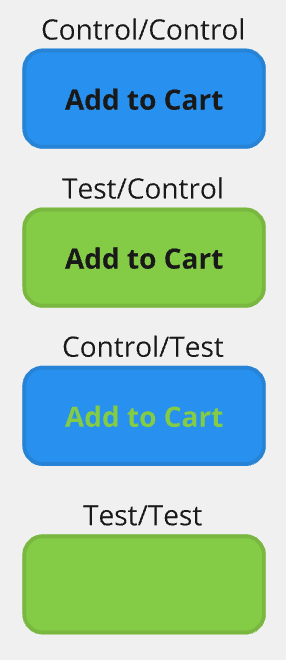
The test/test combination, in particular, is pretty catastrophic - I would expect a huge drop in Add to Cart clicks in this group. While this sort of clash seems obvious to detect (just look at the button), bear in mind that firstly, most experiments are way more subtle, and clashes are not necessarily visual, and secondly, from the perspective of an experimenting team, it is almost impossible to determine which of your sessions are in the other experiment’s test group. Even if the experimenter actually visits the site, they only have a 25% probability of being assigned to the ‘dud’ combination.
Ok, let’s talk about the impact that this might have. Imagine our control/test splits are 50/50, and that the baseline click rate is 10% - that is, 10% of sessions have an Add To Cart click in them absent any experiments. It’s the ‘rate in the wild’. Let’s say the Button Experiment has a true click rate of 15%, the Font Experiment has a 12% true click rate, the colliding test groups have a 2% click rate, and that these experiments are exposed to 1 million sessions.
If the sessions are truly randomly assigned, we can expect to see 250000 sessions in control/control, 250000 in test/control, 250000 in control/test and 250000 in test/test. If these experiments were run in isolation, we would conclude that the Button Team experiment has the greatest click rate, followed by the Font Team experiment, followed by the Baseline.
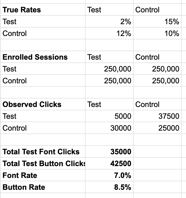
Unfortunately, each of these teams will be including the test/test results in their session counts, which dramatically skews their results. As you can see in the workings above, the Button Team concludes that their click rate is 8.5%, the Font Team conclude that their click rate is 7% - just because of that tainted 25%.
Since these scores are both lower than the baseline of 10%, no permanent change will be made to the site, and the company misses out on a potentially 50% increase in cart additions.
Testing for metric interaction
There are a few methods for detecting interaction between two experiments. We make use of the regression method. Basically, this method involves the following steps:
1. Arrange your session data such that you have one row per session, one column per experiment and one column for your metric
Each experiment column can have only three possible values:
- We assign a NULL if the session was not enrolled in the experiment.
- We assign a 0 if it was enrolled in the experiment and assigned to control - that is, nothing new is shown to it.
- We assign a 1 if it was assigned to the session and assigned to test - that is, it is shown the change.
The metric column can take any value. It represents the outcome of that session according to what you care about. For example, an add_to_cart column would have TRUE/FALSE values; a revenue column would have a decimal larger than or equal to 0.00.
Here is a synthetic example of such a table:
>>> df
        end_date  offer_1  offer_2   revenue
0     2024-09-02        1        1     0.000
1     2024-09-02        1        0     0.000
2     2024-09-02        0        0     0.000
3     2024-09-02        1        1     0.000
4     2024-09-02        1        1   131.210
...          ...      ...      ...       ...
99995 2024-09-02        0        1     0.000
99996 2024-09-02        1        1   137.027
99997 2024-09-02        1        0   112.610
99998 2024-09-02        1        0     0.000
99999 2024-09-02        1        1   110.935

[100000 rows x 5 columns]
2. Create a regression that treats a metric as the dependent variable, the two experiments as independent variables, and the presence of both of the experiments as a third independent variable.
This third variable is known as an interaction term, and is pretty standard practice in regression analysis. The formula for such a model is will look something like this:
model = ols(f"revenue ~ offer_1 * offer_2", data=df)
3. Evaluate the p-value of the interaction term
The results of the regression will look something like this (you might want to view on a wide screen):
results = model.fit()

>>> results.summary()
<class 'statsmodels.iolib.summary.Summary'>
"""
                            OLS Regression Results
==============================================================================
Dep. Variable:                revenue   R-squared:                       0.124
Model:                            OLS   Adj. R-squared:                  0.124
Method:                 Least Squares   F-statistic:                     4707.
Date:                Mon, 02 Sep 2024   Prob (F-statistic):               0.00
Time:                        14:24:42   Log-Likelihood:            -5.3290e+05
No. Observations:              100000   AIC:                         1.066e+06
Df Residuals:                   99996   BIC:                         1.066e+06
Df Model:                           3
Covariance Type:            nonrobust
===================================================================================
                      coef    std err          t      P>|t|      [0.025      0.975]
-----------------------------------------------------------------------------------
Intercept       -2.586e-11      0.316  -8.19e-11      1.000      -0.619       0.619
offer_1            41.7501      0.445     93.776      0.000      40.878      42.623
offer_2            46.2747      0.447    103.540      0.000      45.399      47.151
offer_1:offer_2   -46.8251      0.631    -74.179      0.000     -48.062     -45.588
==============================================================================
Omnibus:                    13274.097   Durbin-Watson:                   2.010
Prob(Omnibus):                  0.000   Jarque-Bera (JB):            19272.982
Skew:                           1.064   Prob(JB):                         0.00
Kurtosis:                       3.305   Cond. No.                         6.85
==============================================================================

Notes:
[1] Standard Errors assume that the covariance matrix of the errors is correctly specified.
"""
Ok, that looks super intimidating. We actually only care about one line of the output:
                      coef    std err          t      P>|t|      [0.025      0.975]
offer_1:offer_2   -46.8251      0.631    -74.179      0.000     -48.062     -45.588
What does this mean? Well, this is the line that tells us about the contribution that the interaction term makes to the predicted value of revenue. We are particularly interested in the value
P>|t|
0.000
What this tells us is that, to a very high degree of certainty (anything less than 0.05 is 95% significant, anything less than 0.01 is 99% significant), the interaction term contributes meaningfully to the predicted value of revenue. Simply put, the presence of both experiments moves the needle in a way that is additive to the predictive power of the presence of offer_0 or offer_1 in isolation.
Therefore, we can conclude that there is evidence of interaction between these two experiments.
Pretty simple, huh?
OK but how how do you deal with more than two experiments?
Well, if you have in the order of, say, 50 experiments running simultaneously, you need to do a regression for each pair independently. That’s about 1225 regressions. If you are testing for multiple metrics, you are looking at 1225 regressions per metric. We run these regressions in parallel, and add the results of each regression to a dictionary that we then coerce to a dataframe. We then write this dataframe back to our warehouse for downstream beutification and visualisation. Here is the rough structure of our metric interaction results dataframe. I have printed samples from each column to a separate line to save you from more wide-screen blues:
>>> glimpse(metric_results)
Rows: 6
Columns: 14
$ test_time <datetime64[ns, UTC]> ['2024-09-02T14:00:00.000000000' '2024-09-02T14:00:00.000000000'
$ measure <object> ['revenue' 'purchase' 'purchase']
$ exp_x <object> ['offer_1' 'offer_2' 'offer_1']
$ exp_y <object> ['offer_2' 'offer_3' 'offer_2']
$ num_observations <int64> [100000 100000 100000]
$ corr <float64> [-0.00262683  0.00446337 -0.00262683]
$ sample_exp_x_1_mean <float64> [41.47704491  0.42603836  0.41455873]
$ sample_exp_y_1_mean <float64> [43.7373768   0.41931909  0.42603836]
$ sample_exp_x_0_mean <float64> [23.07887879  0.39595686  0.40726259]
$ sample_exp_y_0_mean <float64> [20.98305848  0.40063618  0.39595686]
$ interaction_p_value <float64> [0.00000000e+00 2.46952290e-18 1.24672431e-02]
$ interaction_coefficient <float64> [-4.68251233e+01  5.45876152e-02  1.55426521e-02]
$ interaction_std_error <float64> [0.6312481  0.00624918 0.00622034]
$ interaction_t_value <float64> [-74.17863597   8.73516848   2.49868086]
One can filter the above table for results where the interaction_p_value fall below a desired threshold. These are you clashing experiments. You can get hold fo those teams and notify them of the issue, and devise a way to re-run those experiments again to obtain un-skewed results.
It’s important to note that, because we are running many independent regressions, there is the possibility that the interaction_p_value is an accident. We can expect that, as a P value threshold of 5%, 5% of our P value estimates can be wrong. So we could detect interaction effects where there are in fact none. To deal with this, one should consider applying an adjustment to the P value after the fact (we chose the Bonferroni correction for its simplicity, but there are others).
OK but what about performance?
If you are running these evaluations regularly for a large site, you need to think about processing speed.
On any evaluation run (we do 3 a day), we evaluate 14 days of data (about 50m sessions), about 50 experiments, three metrics, and we also do a traffic interaction effect test. This amounts to about 5000 independent statistical tests, run against a 50m row dataset, and we have gotten runtime down to about four and a half minutes, on a node that uses about 3gb of RAM and four threads.
Initially we tried to implement a regression in pure SQL - mostly to keep everything in our data warehouse, but also because then we wouldn’t have to take on the technical debt of another programming language. This is quite valuable to us.
But it quickly became clear that doing this in SQL would result in huge costs and take huge amounts of time. So, we decided to put the creation of the regression table in SQL, but to pull it down to a local node to conduct the regressions in python. We then push the results tables back up to BigQuery to be picked up by downstream data pipelines.
Here is an incomplete list of our findings as we roughed out our process:
- Exporting a large BigQuery table to parquet and pulling that is way cheaper (in time and compute) than a direct SQL to dataframe query.
- Loading the full regression frame to memory would take (we estimate based off samples) about 400GB of RAM, but each experiment pair of columns takes about 2gb of RAM. So reading from disk for each regression is way cheaper.
- Reading selected columns from parquet to pandas takes about a factor of 5 longer than loading the whole table from parquet to duckdb, and then querying duckdb for the selected columns.
- Pre-sorting our BigQuery regression table in order of ‘most experiment heavy’ sessions reduced load time by 30%, presumably because the duckdb engine needs to read less blocks to retrieve data (lots of the blocks will just have NA for all rows for a particular pair).
- duckdb multiprocessing is marginally faster than multithreading, but much more complex to implement.
- Because the multi regression problem is embarassingly parallel, more threads reduces overall compute time really efficiently.
- The data read operation takes about 95% of the total compute time for a particular test. The actual regression operations are really fast.
- We tried to put the persistent duckdb file on a ramdisk, but it made no appreciable speed increase over storage on a persistent disk. We therefore think that the read operation is not IO bound, it is CPU bound - probably the decompression operation.
So, our cheapest-and-quickest run path ended up being (in my made up pseudocode)
BigQuery -> gcp/table{0-n}.parquet -> local disk -> duckdb

begin loop {1:combinations(experiments)}
    duckdb -> pandas -> statistical computations -> append to results dictionary
end loop

results dictionary -> dataframes -> BigQuery tables
Summing up
Ok, that was quite a lot of information. I hope that you now:
- Understand how an AB test is structured
- Can see the impact that experiment interaction can have on experiments
- Understand how to use regression analysis to check for metric interaction
- Have a rough sketch of how this might be turned into a large scale operation, and what sort of performance tradeoffs you might need to make.